How Does Mean And Standard Deviation Change

A plot of a normal distribution (or bell curve). Each colored band has a width of one standard difference.

A data set up with a mean of 50 (shown in blue) and a standard deviation (σ) of 20.

Example of 2 sample populations with the same mean and different standard deviations. Cherry-red population has mean 100 and SD 10; blue population has hateful 100 and SD fifty.

Standard deviation is a number used to tell how measurements for a group are spread out from the average (hateful or expected value). A low standard deviation means that most of the numbers are shut to the average, while a loftier standard deviation means that the numbers are more spread out.^{[one] [2]}

The reported margin of error is usually twice the standard deviation. Scientists unremarkably report the standard difference of numbers from the average number in experiments. They often decide that only differences bigger than two or iii times the standard deviation are important. Standard divergence is also useful in coin, where the standard deviation on involvement earned shows how different one person'south interest earned might be from the average.

Many times, only a sample, or part of a group can be measured. So a number close to the standard deviation for the whole grouping can be constitute by a slightly dissimilar equation called the sample standard deviation, explained beneath. In which case, the standard divergence of the whole group is represented by the Greek letter ${\displaystyle \sigma }$ , and that of the sample by ${\displaystyle south}$ .^[3]

Basic example [change | change source]

Consider a grouping having the post-obit viii numbers:

${\displaystyle 2,\ 4,\ 4,\ 4,\ 5,\ v,\ 7,\ 9}$

These eight numbers have the average (hateful) of 5:

${\displaystyle {\frac {2+4+4+4+5+5+7+ix}{eight}}=v}$

To calculate the population standard deviation, first find the divergence of each number in the list from the hateful. So square the consequence of each difference:

${\displaystyle {\begin{array}{lll}(2-v)^{2}=(-iii)^{ii}=9&&(5-five)^{ii}=0^{2}=0\\(4-v)^{two}=(-1)^{2}=1&&(five-five)^{2}=0^{2}=0\\(4-v)^{2}=(-ane)^{2}=1&&(7-5)^{2}=2^{2}=4\\(4-5)^{two}=(-1)^{2}=1&&(9-v)^{2}=4^{two}=xvi\\\stop{assortment}}}$

Next, discover the average of these values (sum divided by the number of numbers). Last, have the square root:

${\displaystyle {\sqrt {\frac {(9+1+1+ane+0+0+four+xvi)}{8}}}=2}$

The reply is the population standard deviation. The formula is merely true if the eight numbers we started with are the whole group. If they are only a part of the group picked at random, then we can obtain an unbiased estimate of what the population standard deviation is past dividing past 7 (which is n − 1) instead of 8 (which is north) in the lesser (denominator) of the formula above. And then the respond is the (bias-corrected) sample standard deviation.^[iv] This is called the Bessel'due south Correction.^[5] Nosotros oft use this correction because the sample variance, i.e., the square of the sample standard deviation, is an unbiased estimator of the population variance, in other words, the expected value or long-run average of the sample variance equals the population (true) variance. Nevertheless, it is not the instance that the sample standard deviation is an unbiased reckoner of the population standard deviation.[1] Although Bessel's correction is an unbiased estimate of the variance, this estimate does take a higher mean square error than the biased estimate, or in other words, the biased estimate (that is, dividing past n rather than n-1) is on average closer to the true value.

More than examples [change | alter source]

Here is a slightly harder, real-life instance: The average height for grown men in the U.s.a. is lxx", with a standard difference of 3". A standard deviation of iii" means that nearly men (about 68%, assuming a normal distribution) have a height 3" taller to 3" shorter than the average (67"–73") — one standard deviation. Almost all men (about 95%) accept a height 6" taller to 6" shorter than the average (64"–76") — two standard deviations. 3 standard deviations include all the numbers for 99.7% of the sample population being studied. This is true if the distribution is normal (bong-shaped).

If the standard divergence were aught, then all men would exist exactly 70" tall. If the standard divergence were 20", then some men would be much taller or much shorter than the boilerplate, with a typical range of about 50"–90".

For another example, each of the iii groups {0, 0, fourteen, 14}, {0, 6, viii, 14} and {half-dozen, six, eight, 8} has an average (hateful) of 7. But their standard deviations are 7, 5, and 1. The third group has a much smaller standard deviation than the other 2 because its numbers are all close to vii. In general, the standard divergence tells united states how far from the boilerplate the rest of the numbers tend to be, and information technology will take the aforementioned units as the numbers themselves. If, for case, the group {0, half-dozen, 8, 14} is the ages of a group of four brothers in years, the boilerplate is 7 years and the standard deviation is 5 years.

Standard difference may serve as a measure of uncertainty. In science, for instance, the standard divergence of a group of repeated measurements helps scientists know how sure they are of the average number. When deciding whether measurements from an experiment agree with a prediction, the standard deviation of those measurements is very important. If the average number from the experiments is besides far abroad from the predicted number (with the altitude measured in standard deviations), then the theory being tested may non be correct. For more information, see prediction interval.

Awarding examples [change | change source]

Understanding the standard deviation of a set of values allows us to know how big a divergence from the "boilerplate" (mean) is expected.

Weather [change | modify source]

Equally a unproblematic example, consider the average daily high temperatures for two cities, ane inland and one near the ocean. It is helpful to empathize that the range of daily loftier temperatures for cities nigh the ocean is smaller than for cities inland. These two cities may each take the same average daily loftier temperature. However, the standard deviation of the daily high temperature for the littoral city volition be less than that of the inland urban center .

Sports [modify | change source]

Another way of seeing it is to consider sports teams. In whatsoever sport, there volition be teams that are skillful at some things and not at others. The teams that are ranked highest volition non show a lot of differences in abilities. They practice well in most categories. The lower the standard deviation of their ability in each category, the more counterbalanced and consequent they are. Teams with a higher standard deviation, yet, volition be less anticipated. A team that is usually bad in most categories will have a low standard divergence. A squad that is normally good in virtually categories will also have a low standard deviation. However, a squad with a high standard divergence might exist the type of team that scores many points (stiff offense) but also lets the other team score many points (weak defense).

Trying to know ahead of fourth dimension which teams will win may include looking at the standard deviations of the various team "statistics." Numbers that are different from expected can match strengths vs. weaknesses to show what reasons may be well-nigh important in knowing which squad will win.

In racing, the fourth dimension a driver takes to finish each lap around the track is measured. A driver with a low standard deviation of lap times is more consistent than a commuter with a higher standard deviation. This information can be used to help understand how a driver tin reduce the time to stop a lap.

Money [change | alter source]

In money, standard deviation may hateful the take a chance that a price will go upwards or down (stocks, bonds, property, etc.). It can as well hateful the risk that a group of prices volition go upward or downwardly^[six] (actively managed common funds, index mutual funds, or ETFs). Take a chance is one reason to make decisions about what to buy. Risk is a number people tin use to know how much money they may earn or lose. Equally risk gets larger, the render on an investment can be more than than expected (the "plus" standard divergence). Even so, an investment tin can also lose more money than expected (the "minus" standard difference).

For example, a person had to choose between 2 stocks. Stock A over the past twenty years had an average return of x percent, with a standard deviation of twenty percentage points (pp). Stock B over the past xx years had an average return of 12 percent but a higher standard deviation of 30 pp. Thinking nearly the risk, the person may decide that Stock A is the safer choice. Even though they may not brand as much money, they probably will non lose much money either. The person may think that Stock B's 2 point higher average is not worth the additional ten pp standard deviation (greater risk or incertitude of the expected return).

Rules for normally distributed numbers [alter | change source]

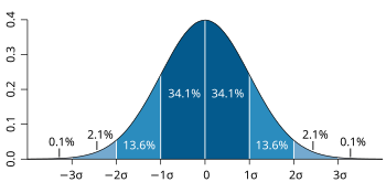
Dark blue is less than ane standard deviation from the mean. For the normal distribution, this includes 68.27 percent of the numbers; while two standard deviations from the mean (medium and night bluish) include 95.45 pct; 3 standard deviations (light, medium, and night blue) include 99.73 pct; and four standard deviations account for 99.994 pct.

Almost math equations for standard divergence assume that the numbers are normally distributed. This means that the numbers are spread out in a certain way on both sides of the boilerplate value. The normal distribution is besides called a Gaussian distribution because it was discovered by Carl Friedrich Gauss.^[7] It is often chosen the bell curve because the numbers spread out to make the shape of a bong on a graph.

Numbers are not ordinarily distributed if they are grouped on ane side or the other side of the boilerplate value. Numbers tin be spread out and notwithstanding exist normally distributed. The standard deviation tells how widely the numbers are spread out.

Relationship between the average (mean) and standard deviation [change | change source]

The average (mean) and the standard divergence of a set up of data are commonly written together. Then a person can empathize what the average number is and how widely other numbers in the group are spread out.

The fashion a group of numbers is spread out can also be given by the coefficient of variation (CV),^[iii] which is the standard deviation divided by the average. Information technology is a dimensionless number. Coefficient of variation is often multiplied past 100% and written as a pct.

History [alter | change source]

The term standard deviation was first used in writing by Karl Pearson in 1894,^{[8] [9]} after he used information technology in lectures. It was equally a replacement for before names for the aforementioned idea: for example, Gauss used mean error.^[ten]

[alter | alter source]

• Accuracy and precision
• Sample size
• Standard error
• Variance

References [modify | alter source]

1. ↑ Gauss, Carl Friedrich (1816). "Bestimmung der Genauigkeit der Beobachtungen". Zeitschrift für Astronomie und verwandt Wissenschaften. 1: 187–197.
2. ↑ Walker, Helen (1931). Studies in the History of the Statistical Method. Baltimore, Doctor: Williams & Wilkins Co. pp. 24–25.
3. ↑ ^{3.0 3.1} "Listing of Probability and Statistics Symbols". Math Vault. 2020-04-26. Retrieved 2020-08-21 .
4. ↑ Weisstein, Eric Due west. "Standard Difference". mathworld.wolfram.com . Retrieved 2020-08-21 .
5. ↑ "Standard Divergence Formulas". www.mathsisfun.com . Retrieved 2020-08-21 .
6. ↑ "What is Standard Deviation". Pristine. Retrieved 2011-10-29 .
7. ↑ Kirkwood, Betty R; Sterne, Jonathan AC (2003). Essential Medical Statistics. Blackwell Science Ltd. {{cite volume}}: CS1 maint: multiple names: authors list (link)
8. ↑ Dodge, Yadolah (2003). The Oxford Dictionary of Statistical Terms. Oxford Academy Printing. ISBN0-nineteen-920613-ix.
9. ↑ Pearson, Karl (1894). "On the autopsy of asymmetrical frequency curves". Phil. Trans. Roy. Soc. London, Series A. 185: 719–810.
10. ↑ Miller, Jeff. "Earliest known uses of some of the words of mathematics".

Other websites [change | change source]

• A simple way to understand Standard Deviation
• Standard Departure – an explanation without maths
• Standard Departure, an uncomplicated introduction
• Standard Deviation, a simpler explanation for writers and journalists

Source: https://simple.wikipedia.org/wiki/Standard_deviation

Posted by: pickettofeautioull.blogspot.com

Share this post